Sun is the fundamental source of energy, which heats the atmosphere and creates air motions. These air motions distribute heat and moisture in the atmosphere and weather systems are created whenever energy from sun combines with moisture. Hence, weather pertains to a state of the atmosphere that is experienced at a given time (also reported at synoptic hours) that is defined by variables such as temperature, pressure, winds, rainfall, cloud cover (expressed in octas) and several other dynamical and thermodynamical variables. But, climate is the mean state of the atmosphere that arises from interplay of meteorological processes that constantly change the state of the atmosphere in motion. Thus, climate would refer to averages of weather elements obtained from their time series for a location or any region. In effect, the climate could imply monthly, seasonal or annual mean distributions of temperature, rainfall or for that matter of any other weather element of interest, depending on the averaging period. In this sense weather and climate are intimately linked together. The day-to-day variations in weather if persist for longer periods, leave invariably their footprints in the climate of a place or region. Putatively, climate could also refer to the probability of occurrence of a particular type of weather regime during a particular period of the year to which the reference has been made. To illustrate this point, consider the monsoon rainfall in India. The country receives nearly 75% of its annual rainfall during the 120-day long monsoon season (June-September). The forthwith interpretation could be that the probability of rain water falling everyday during the monsoon season could be 75% of the daily All-India mean rainfall (temporal sense); or on the country scale, 75% area of the country has the probability of receiving average rainfall (spatial sense) daily in this 120-day period. Obviously, predictions based on persistence have high failure rate which brings into prominence the role of numerical weather prediction models. Nevertheless, the persistent structures in the ever-evolving patterns of atmospheric variables have to be studied for climate analysis; the variance of these variables from their weakly, monthly, seasonally or annually persistent structures precisely indicates the climate variability on the corresponding scales. The above description may however imply that the climate depends only on atmospheric processes. If accepted in totality, it would be misleading. Essentially, the interaction of the climate with other processes and components of the earth system gives rise to feedbacks that significantly influence the response of the climate system. For example, the variations in the solar constant and the human-induced changes in the composition of the atmosphere would secularly affect the radiative balance of the earth system and its climate; that is, the climatic response would either amplify or dampen under the influence of any such imposed external forcing.
Since atmospheric models are backed by highly advanced data assimilation systems, major forecasting centres nowadays are issuing seasonal forecasts. With coupled ocean-atmosphere models, longer forecasts out to a decade are also possible and are being indeed produced to predict phenomena arising from interaction of atmospheric and oceanic processes, such as El Niño and Southern Oscillation. Such models require huge resources, computing power and analyses prepared from global atmospheric observations and ocean data of several years. Our understanding of the climate system has grown steadily as a result of success in numerical simulations of weather and climate as well as from careful process studies under three different fields, viz., meteorology, oceanography and aeronomy, which practically developed independently of each other.
It is the science of atmosphere that deals with the changing patterns of heat, moisture and air motion in the three dimensional space, which can be described by physical laws. Understanding the behaviour and distribution of heat and moisture is the key to understanding weather systems that can also be probed by ground-based instruments and satellite observations. The pressure and wind systems on the synoptic scale are analysed for weather prognosis; hence weather charts have played a central role in synoptic forecasting of weather though it has limited range of validity. Sir Gilbert Walker, however, invented statistical methods to make a long-range forecasting of monsoon rainfall. Such forecasts for the All-India summer monsoon rainfall have been successful for the country as a whole nearly for a century, though district-wise rainfall forecast with such techniques turns out to be very difficult. Now, weather predictions are accurately made up to 10 days in advance by assimilating conventional meteorological (mostly radiosonde) data and satellite radiances directly into more sophisticated high-resolution three-dimensional dynamical models, which also serve as tools of climate and climate change simulations. Interestingly, meteorology evolved with the theory that successfully explained the advent of summer monsoons over India by Hadley (1857).
It is the study of The Real Ocean often described as complex, dilute solution of extremely large volume of waters where several chemical reactions are taking place. In response to energy received from the atmosphere or through the atmosphere (i.e. solar radiation), circulations at various temporal and spatial scales characterize the ocean state. The ocean currents transport waters with dissolved material from one place to another. The life forms in the ocean depend upon the chemistry of their environment. Their distribution and productivity are determined by circulation and physical properties of ocean waters. However, for a complete understanding, the biology, chemistry, geology, and physics of the oceans must be known. Like atmosphere, ocean observations too are key to understanding oceanic phenomena and ocean currents. The ocean observations are compiled and preserved as hydrographical data that provide information on water depths, shorelines, tides, currents, bottom types, undersea ridges, valleys and other features in the realm of ocean.
As a subject, it deals with the study of atmospheres of planets; therefore, it encompasses topics like air chemistry, aerosols, clouds and radiation, and troposphere-stratospheric interactions. The middle atmosphere extending from 10-16 km to 100 km has been thoroughly investigated by aeronomists. The ozone problem has been at the heart of this subject, which led to the stratospheric ozone recovery strategies by successfully identifying the chemicals that are responsible for the destruction of ozone. Several nations united to protect the ozone layer once the ozone hole was discovered over Antarctica, which is as large as the size of North America during a given astral spring. The global warming induced by greenhouse gases (GHG) is currently the key topic of research and development of GHG emission control technologies. In the present day numerical prediction models, ozone is assimilated in the analysis like any other conventional weather parameter. The transboundary pollutant transport is one of the key concerns of today as NOx, SOx and other pollutants once emitted in the atmosphere disperse globally and trigger complex chemical reactions under the prevailing atmospheric conditions to form new particles which on ageing become cloud condensation nuclei that impact the growth and reflectivity of clouds, and precipitation intensities. It is worth pointing out that aerosols produce both direct (scattering of incoming solar radiation) and indirect forcing (through cloud albedo enhancement and inhibition of precipitation from clouds) on climate. The chemical reactions in the lowest layers (troposphere and stratosphere) are the focus of climate change research. The middle atmosphere dynamics that successfully explained the sudden stratospheric warming and quasi-biennial oscillations (QBO) in the stratosphere is at the core of aeronomy.
For understanding weather and climate of the earth, observations on weather elements are of paramount importance. Temperature and wind are daily measured at regular intervals. The balloon flights carrying radiosondes aloft provide accurate description of thermodynamic variables like temperature, pressure and moisture. Satellite observations provide finer structure and high-resolution spatial (one kilometre) and temporal (half-hourly) details of temperature and moisture fields horizontally and, in general, of the atmospheric circulation. Ocean temperatures are measured by travelling ships and by sensors deployed in ocean waters and on satellites. While radiosondes provide records of atmospheric temperature, humidity and pressure distribution in the vertical, drifting floats make continuous measurements of salinity (conductivity), temperature and pressure (depth) in the ocean. These floats, also called the “floating CTDs”, make same measurements that a Conductivity-Temperature-Depth (CTD) sensor does. They have the ability to sink typically to a depth of 2,000 metres in the ocean by changing their buoyancy and remain 7-10 days at that depth while continuously drifting with the ocean currents. By again changing their buoyancy, the drifting floats come to the surface and transmit the time of observations, position in the ocean and profiles of ocean variables to the orbiting satellites. These floats are indeed the marvels of technology and form the backbone of the Argo Programme in the global ocean. There are more than 3000 Argo floats that are active globally; roughly 10% of them are deployed in the Indian Ocean. In this course, we shall deal with physical oceanography that concerns to physical properties and processes within the ocean depths, and some conceptual models of ocean dynamics in order to explain surface currents and their relation to buoyancy and mixing.
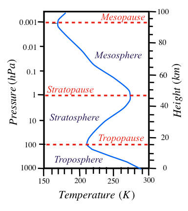
The planet Earth is unique in the Solar System for sustaining life due to the presence of water and oxygen with several other gaseous constituents prominent among them being nitrogen, carbon dioxide and ozone in its atmosphere. Water exists in all three forms (solid, liquid and gas) on earth and transformation of water vapour into liquid form as cloud drops in the atmosphere, produces life giving rains falling back onto surface. Ozone absorbs the ultra-violet radiation from Sun and thus protects the lives of humans and animals on this planet from potential damages. The atmospheric pressure decreases with height but temperature shows strong variations (Fig. 1.1) in the vertical, typically increasing or decreasing linearly in a particular atmospheric layer. The temperature decreases linearly with height in the lowest atmospheric layer (called the troposphere) from surface to 10 km altitude and then increases in the “stratosphere” up to an altitude of 50 km.
The gradient of temperature in the vertical (or lapse rate) changes its sign from negative to positive in the “tropopause” region at about 10 km (100 hPa) above the ground (Fig. 1.1), whereas the opposite happens (i.e. from positive to negative) in the “stratopause” region located at about 50 km (1 hPa) above the ground. Thus 99.0% of the mass of the atmosphere resides in the gaseous envelope extending from surface up to 50 km height that surrounds the planet earth. The region above 50 km is known as the “mesosphere” which is topped by the “mesopause”, and the atmospheric pressure has reduced there to 0.001 hPa. The middle atmosphere refers invariably to both stratosphere and mesosphere that extends from tropopause to a height of 85 km.
Figure 1.1 Variation of mean temperature (K) with height up to an altitude of 100 km in the atmosphere (Fleming et al. 1990). Temperature decreases in troposphere (lapse rate = 10K/km (dry); 6.5K/km (moist)) with height, and increases in stratosphere attaining maximum at the stratopause (~ 50 km). These two layers together contain 99% of mass of the atmosphere. |
 |
|---|
Like in altitude, atmospheric temperatures also show strong variations from equator to pole: warmest at equator and coldest at the poles. The zonally averaged temperatures (that is, the mean temperature of each latitude circle) plotted as a function of latitude and altitude can therefore depict a more complete thermal structure (Fig. 1.2) of the atmosphere. From Fig. 1.2, it may be noted that the tropopause level is highest in the tropics (30S, 30N) reaching up to about 16 km due to intense convective overturning in the equatorial region with coldest temperatures (200 K). However, its height is about 8 km over poles (absence of convective overturning) with temperatures 10 - 20 K warmer than those over the equatorial region even during perpetual darkness of winters over poles. At this level, an abrupt change in temperature (or lapse rate) may be noted both in Polar Regions and the Tropics; that is, temperatures decrease with altitude below the tropopause and rise above this level. However, such an abrupt change is not seen in the mid-latitudes, which is evident from breaks in the tropopause (Fig. 1.2) both in the southern and northern hemispheres. Winds with intense shear, are strongest in these regions attaining jet speeds (50 ms-1 and above) at 200 hPa over southeastern United States, Mediterranean Sea and Japan are referred to as the jet streams.
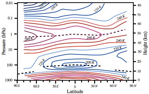
Figure 1.2 Height-latitude cross-sections of zonal-mean atmospheric temperatures (K) during northern winter. The dashed lines show tropopause (100 hPa) and stratopause (1 hPa) where lapse rate abruptly changes. Note also breaks in the tropopause at mid-latitudes. (Temperature above 80 km, refer Fleming et al. (1990)
The concentration of atmospheric constituents varies in the vertical (i.e. it is a function of altitude). For example, the distribution of zonal mean water vapour mixing ratio shows that it is very much confined to the troposphere with maximum amounts (20 g/kg) at the surface falling off rapidly with altitude in the lower troposphere (Fig. 1.3).
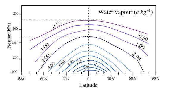
Figure 1.3 Variation of zonal mean water vapour mixing ratio with latitude and pressure. Shaded area represents 60% of the maximum value. Mixing ratios superior to 18 g/kg are at surface and 8 g/kg at about 800 hPa (~ 2 km) in tropics as found by Oort and Pexito (1983).
The water vapour mixing ratios fall off below 4 g/kg beyond 60 degree latitude poleward horizontally and above the boundary layer in the vertical apart from tropics. Exceptions are the cloudy regions where water vapour mixing ratios are high. For example, deep convective (cumulonimbus) clouds in tropics can penetrate the entire depth of the troposphere with their bases above boundary layer and cloud tops reaching up to tropopause (Fig 1.4). Thus, the largest fraction of high clouds forms in the tropics. Water vapour mostly originates over warm equatorial ocean waters due to evaporation and transported by the winds to other regions. One of the most illustrative examples of such a kind of transport phenomena is the summer monsoon, which visits the Indian subcontinent every year and remains active for about four months producing a quantum jump in its daily rainfall. Vast amounts of moisture that originate over the southern Indian Ocean (moisture source region) are transported by the monsoon current to produce copious rains over India (moisture sink region). Since water vapour is an efficient absorber of the terrestrial radiation, the patterns of outgoing longwave radiation (OLR) and water vapour (Fig. 1.4 a, b) match very closely. However, ozone is mainly concentrated in the stratosphere and mesosphere (Fig. 1.5). The maximum ozone number density (number of molecules per cubic metre) is in the stratosphere, a stable layer often referred to as the “ozone layer” in the atmosphere.
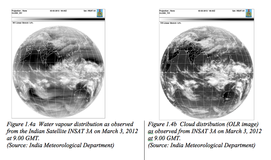
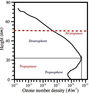
Figure 1.5 Vertical profile of ozone number density (# of molecules per cubic metre) from U.S. Standard Atmosphere (1976). Dominant levels of O3 may be noted in the stratosphere (the ozone layer) and it is present in the atmosphere up to a height of 70 km. Thus bulk of the O3 is present in the middle atmosphere (stratosphere and mesosphere). Ozone concentration is maximum at a height of 22 km but temperature (Fig. 1.1) is maximum at the stratopause level (~50 km).
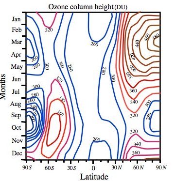
Figure 1. 6 The observed annual cycle of column ozone in the 5-year climatology of Li and Shine (1995). Column ozone amounts are in Dobson Unit (DU). O3 peaks in NH high latitudes (480DU) and SH middle latitudes (360 DU) during spring. Note the Ozone Hole over the Antarctica with low O3 concentrations (200 DU). 1 DU = 1/100 mm of column ozone 1 DU = 2.6 ×10²⁰ molecules O3 cm-2.
Another distinctive feature of column ozone distribution could be noted during Antarctic spring (September-October) when column ozone drops to alarmingly low values over the South Pole (200 DU), a manifestation of the “Antarctic ozone hole” discovered by J.C. Farman, B.G. Gardiner and J.D. Shaklin, which was largest in September 2006. This dramatic reduction of ozone in the stratosphere over Antarctica has been found to be the result of loss of ozone, which happens due to complex chemical and physical processes, involving chlorine from chlorofluorocarbons (CFCs), on the ice particle which can form in extremely low temperature in this region. Although the ozone levels rise later in the year but the Ozone Hole over Antarctica became the subject of intense theoretical and observational studies and international efforts paved the way for phasing out the use of CFCs in accordance to the Montreal Protocol and later the Kyoto Agreement on the reduction of emission of greenhouse gases to save the planet from the potential damages of global warming.
Carbon dioxide, a major greenhouse gas of global concern, is well mixed in the atmosphere. Most of the atmospheric CO2 (397 ppm) is used up by plant life through the photosynthesis process. Thus, oceans also absorb carbon dioxide due to the ubiquitous presence of phytoplankton in saline waters that are grazed by zooplanktons feeding fish. However, the secular increase of CO2 in the atmosphere, evident from (Fig. 1.7), would have far-reaching consequences, as mean atmospheric temperatures would also rise leading to global warming. Excessive absorption of CO2 by oceans can, in effect, change the pH of ocean waters; this could be disastrous to ocean life because some kinds of rare fish and organisms could disappear permanently. For a systematic study of changes in the concentration of atmospheric constituents resulting from chemical transformations,it is necessary to constantly probe the chemical composition of the atmosphere.
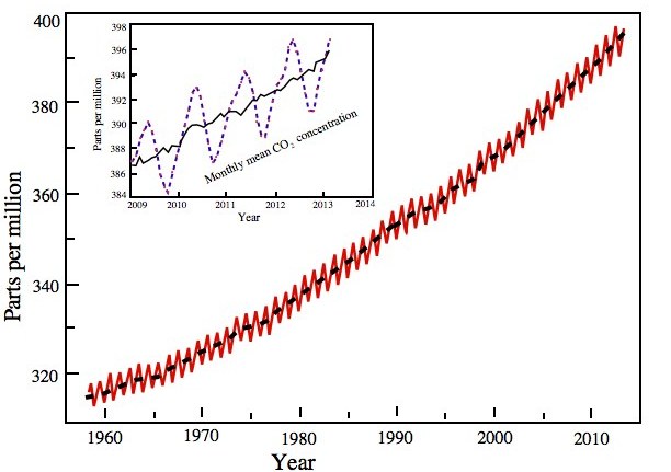
Figure 1.7 Mixing ratio of carbon dioxide over Mauna Loa, Hawaii. The mean annual cycle of CO2 is shown in the inset picture.
The NOAA observations show a secular rise in the levels of carbon dioxide. Note the changing slope in the rise of CO2. Along the x-axis the years are sown and on the ordinate CO2 concentration in parts per million (ppm) is shown.
The composition and physical properties of the atmosphere and ocean are intimately linked to each other due to air-sea interaction at the interface. The age of the earth is estimated to be 4.6 × 10⁹ (4.6 Ga). During the period of cooling which began some 3.8 Ga before present, oceans evolved from precipitation of transitory steam into liquid form during planetary accretion. The present day atmosphere is composed of the chemical species that are abundant in the atmosphere and though some species are present in trace amounts yet play an important role in maintaining the vertical thermal structure of the atmosphere.
The fractional concentration of the chemical constituents in the atmosphere is summarized in Table 1.1 in accordance to the number of molecules or partial pressures (i.e. concentration by volume). In the present times, climate and “climate change” have become important topics of research with past and present observations including proxy data, and by using the numerical models of climate prediction. For understanding the atmosphere, we need to determine its mass and composition that is continuously changing due to the dominant anthropogenic activity. Thus, any change in the concentration of even trace gases (such as ozone) would point to the perils of industrialization and large-scale destruction of vegetation cover or warming of oceans. The state of the atmosphere in motion may however be predicted from an initial state, days and weeks ahead using the laws of nature. But, for climate and climate change, it is necessary to understand the factors that determine the average state of the atmosphere and its interaction (exchange of energy) with the other components of earth system, viz., oceans, cryosphere, biosphere and the landmass over periods of years and centuries. To address our concern about climate change, all components of the earth system have to be considered into a mathematical framework often referred to as a climate model – a coupled land-ocean-atmosphere model. These models are of varied complexity that even includes the changing chemistry of the air but we shall only consider the so-called simple models in these lectures.
Chemical constituent |
Molecular weight | Concentration by volume |
Permanent gases: |
||
Nitrogen (N2) |
28.013 |
78% |
| Oxygen (O2) | 32.00 |
21% |
| Argon (Ar) | 39.95 |
0.93% |
Trace gases |
||
Water vapour (H2O) |
18.02 |
0-5% (highly variable GHG) |
Carbon dioxide (CO2) |
44.01 |
380 ppm (GHG) |
Neon (Ne) |
20.18 |
18 ppm |
Helium (He) |
4.00 |
5 ppm |
Methane (CH4) |
16.04 |
1750 ppm(GHG) |
Krypton (Kr) |
83.80 |
1100 ppb |
Hydrogen |
2.02 |
500 ppb |
Nitrous oxide (N2O) |
56.03 |
300 ppb(GHG) |
| Ozone (O3) | 48.00 | 0-500 ppb(GHG) |
Carbon monoxide (CO) |
28.01 |
120 ppb |
Nitrogendioxide (NO2) |
46.01 |
1 ppb |
| Sulphur dioxide (SO2) | 64.06 | 200 ppt |
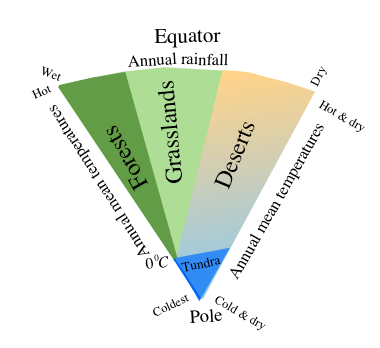
Figure1.8 A conceptual model for displaying the land vegetation types (tundra, forest, grassland and deserts) that will grow depending on the annual rainfall and precipitation over different parts of the globe.Tundra is the treeless region with permanently frozen subsoil water (permafrost). Tundra vegetation includes small shrub like plants and lichens.
The Terrestrial Biosphere refers to the geographical distribution of forests, grasslands, tundra and deserts; their characterization mainly depends on the annual mean temperature and precipitation as shown in Fig. 1.8. For example, tundra on the globe is the dominant treeless region where temperatures even in the warmest month are less than 10°C. Desert vegetation is sparsely distributed in the regions where potential evaporation (proportional to insolation i.e. solar radiation reaching the ground) exceeds precipitation. Depending upon the rainfall amounts received by a particular region, the rest of the land areas on the earth are covered by grasslands and forests. Fig. 1.8 clearly shows that even if water available from precipitation were same for two geographical regions but have different temperatures, then forests would cover regions where mild temperatures prevail in comparison to hot regions that could only sustain grasslands. For a thorough description of the components of the earth system, one may consult the exposition of Wallace and Hobbs (2006) on atmospheric science and other textbooks on this topic.
Ocean is an open system like atmosphere; both ocean and atmosphere can exchange matter across their interface. But the coupled atmosphere-ocean system that they form together is a closed system separated by a common interface. Hence, thermodynamic and dynamical variations in any one component could induce changes in the climate of the whole system through exchanges at the interface. In such a coupled system, ocean is the reservoir of water in the atmosphere and maintains the hydrological cycle of the earth system. In contrast to atmosphere, ocean is opaque to all wavelengths of the solar radiation. Therefore, oceans gain heat in the equatorial latitudes by absorbing solar radiation and lose it mainly due to evaporation. Heat loss from oceans due to evaporation is however reduced in the upwelling regions (along eastern and western African coasts; western American coasts) as cold waters from the thermocline region would lower the sea surface temperatures. For example, Somali current produces strong upwelling that triggers Arabian Sea cooling during the monsoon season; but, on the contrary, if the upwelling on the Peru coast reverses, it marks the onset of a major climatic event, the El Niño, which is the ocean part of the coupled ocean-atmosphere phenomenon, El Niño Southern Oscillation (ENSO). However, cooler than normal temperatures off the coast of Peru are associated with enhanced upwelling due to stronger trades in the region; this event is referred to as La Niña and it is the opposite of El Niño in the ENSO cycle. The ocean currents also play a key role in maintaining the thermal equilibrium of the earth system by transporting heat from equatorial latitudes to Polar Regions in the upper levels and cold waters from pole to equator in deep layers. This gives rise to thermohaline circulation in the ocean on the global scale, which is often referred to as the great conveyor belt in the ocean. It takes thousands of years to complete one cycle. Is there any possibility that the conveyor belt would be switched off in future? This is an important question as it has happened during glaciation in the past. If the conveyor belt switches off, then it would lead to a mini ice age.
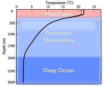
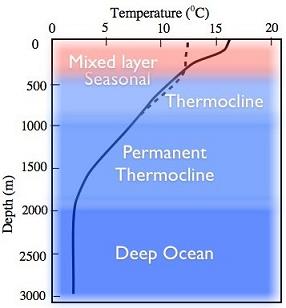
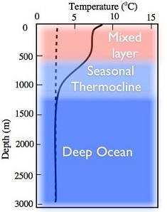
Another key feature of the ocean is its large thermal inertia due to seawater’s large density (1027 kg m-3) and greater specific heat (3986 JK-1g-1) as compared to air. Consequently, it would supposedly delay any possible CO2 induced global warming. Besides, ocean is also a major sink of carbon dioxide. That is why the transfer of atmospheric CO2 to deeper ocean layers by turbulent transfer makes it an important inorganic sink of this greenhouse gas. Moreover, marine plant life too consumes CO2 to transform it into organic material through photosynthesis. Therefore, the abundance of phytoplankton in the ocean renders it an important organic sinkof CO2. Ubiquitous phytoplankton communities in the ocean are nearly responsible for 46% of the planetary photosynthesis. Much of the marine life crucially depends on phytoplankton, which receives nutrients from deeper layers of the ocean. The discussion in the preceding paragraph emphasizes the role of vertical structure of the ocean in the exchange processes and nutrient transport upwards. Like the atmosphere, the vertical structure of the ocean is also inferred from depth wise temperature distribution that is different for tropics (Fig.1.9a), mid latitude (Fig.1.9b) and the polar regions (Fig.1.9c).
 |
 |
 |
|---|---|---|
|
|
|
From the knowledge of the temperature profiles in global ocean basins, it is convenient to divide the oceanic column into three regions (sometimes four when bottom or abyssal waters are included):
- Surface layer (SL): The climate effects on the sea are found in the surface layer as weak gradient from equator to poles with sigma-tee (σt=ρ-1000 kg/m3) increasing with decreasing temperatures. Usually SL is 10-100 m but less than 200 m thick layer except in winters. It is that portion of the ocean column, which experiences seasonal changes in response to the exchange of energy with atmosphere and the absorption of solar radiation. Constant vertical overturning in the ocean mixes temperature (T) and salinity(S); therefore,both these properties are invariant with depth in the so-called “mixed layer”, that is, dq/dz=0, q=(T,S). Consequently, density which otherwise increases with decreasing temperature and increasing salinitywill have uniform vertical distribution (∂ρ/∂z=0) in the mixed layer which is shallower in tropics than in the mid latitude ocean. Hence, it is also referred to as the isopycnal mixed layer. The depth of the 20oC isotherm in the ocean, as shown in Fig. 1.10a, determines the base of the mixed layer and the corresponding depth of the 20oC isotherm as the “mixed-layer depth (MLD)”. However, the 20oC isotherm outcrops at about 40o latitude in both the hemispheres as one may note in Fig. 1.10a; the other isotherms also outcrop as the surface sea temperature decrease. The outcropping of isotherms has important implication on the formation of central waters of the thermocline region where the role of surface wind induced mixing assumes the key role.
- The thermocline (pycnocline) region is below the mixed layer and extends approximately up to a depth of 1000 m where temperatures are in the range of 2- 4oC. It is the region where most rapid decrease in temperature (density) occurs with depth; therefore, density increases downward and it makes the thermocline (TC) region strongly stable. The thermocline waters reach to sea surface due to wind stress forced upwelling in the ocean. The cold waters from the thermocline will reduce sea surface temperatures in the upwelling regions and of other regions where they spread by ocean currents. In this manner, the thermocline participates in the air-sea interaction in global oceans. Moreover, the upward and downward movements of thermocline (pycnocline) have important consequences for the climate especially the event like El Niño often referred to as the El Niño Southern Oscillation (ENSO).
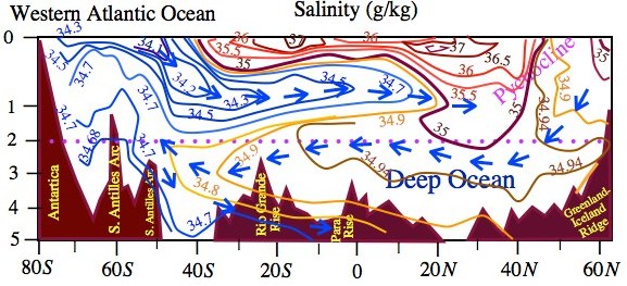
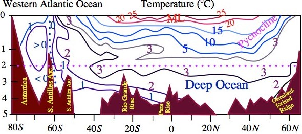
Figure 1.10 Latitude-depth temperature (oC) and salinity in the ocean representing its vertical structure. Thermocline is the layer of strongest vertical gradient in the temperature profile.
- Deep Water (DW) layer is below the permanent thermocline and there is a gradual decrease in temperature and salinity with depth. Usually deep waters are found below a depth of 1000 meters. Deep-water temperatures are below 4oC ; and these waters being isolated from the surface by the stable thermocline, hardly interact with the atmosphere except in the regions on the surface of the ocean where deep waters are formed or destroyed. The depth of the submerged layers varies with latitude: deepest in tropics and shallowest in the high latitudes. Also, sea surface temperatures (SSTs) decrease from the equator to poles; SSTs of about 4oC and cooler would thus be found only in the high latitudes (beyond 50N or 50S). Thus, the isotherms between 0oC and 4oC characterizing deep waters, though remain submerged in tropical and midlatitude ocean depths, would outcrop at sea surface in high latitudes. Due to outcropping of isotherms, cooler surface waters would interact with deep ocean waters in high latitudes. In this manner, deep waters are formed in high latitudes or marginal seas.
Much of the information on the structure of the ocean waters is seen in the two-dimensional cross-sections of temperature and salinity as shown in Fig. 1.10, which represents the structure of the Western Atlantic Ocean. The 20cC isotherm runs at a depth of about 100 m from 30S to 40N suggests that the mixed layer extends beyond tropics in the north. The expansion of mixed layer with its depth exceeding 100 m poleward beyond 30N (Fig. 1.10a) in the North Atlantic is the result of thermal overturning due to evaporative cooling and mechanical overturning by surface winds in the storm tracks. Another interesting feature of the ocean thermal structure is seen in the thermocline region, which is below the mixed layer only in the tropics. The outcropping of isotherms of the thermocline region may be noted in the midlatitude (300-500). The same feature is also seen for the isotherms below 4oC , which characterize deep waters in the ocean. The latitude-depth cross-sections of salinity (Fig. 1.10b) shows that the low salinity water from the 40S – 60S flow down below the mixed layer and a front moves towards equator at a depth between 500 m to 1 km. Another notable observation from this figure is that the thermocline is relatively shallow in the Southern Hemisphere (depth < 1 km) as compared to the Northern Hemisphere where the 4oC isotherm is running at a depth of 1.5 km (Fig. 1.10a).
Since the isotherms in the thermocline region south of the equator are almost straight, therefore, with reference to the equatorward moving density front below the mixed layer, low-density waters are upstream and high-density waters downstream. This sort of horizontal density variations could cause strong mixing in the region where isopycnal lines slope, which can be inferred from the analogy that isopycnal lines dρ/dt=0 in the ocean are like isentropes dθ/dt=0 in the atmosphere. From Fig.1.10b, one can also notice that in the north Atlantic region the heavier waters subduct to a depth of about 3 km and move southwards. The tongue of anomalously dense waters spreads beyond 40S at 3000 m depth. On traversing such huge distances at a speed of less than 1 mm/s (also difficult to measure), the dense waters from north Atlantic finally overrides much heavier waters formed in the Weddell Sea in the south. The deep waters then drift eastward to move around Antarctica and a part of which drifts northwards in the Indian Ocean and through upwelling the nutrient-rich deep cold waters find their way into shallower depths of this basin in about 2000 years.
The density of seawater depends on temperature and salinity, thus it is important to know the composition of seawater besides the temperatures. Major constituents of seawater are salts in the ionic state, which are believed to have come from the weathering of continental rocks. However, more accurate methods of analysis reveal that river waters possess potassium, magnesium, calcium and sodium ions, but they are deficient in dissolved carbon dioxide, chlorides, bromides and iodides. Hence, constituentsof seawater have different sources: potassium, magnesium, calcium and sodium ions come from continental rocks mostly transported by rivers; dissolved carbon dioxide (carbonates, bicarbonates), chlorides, bromides and iodides have originated from volcanic and hot spring discharges into the sea, and from atmospheric sources. These ions are lost constantly by sedimentation on the ocean floorand through transfer to the atmosphere and biosphere. Therefore, there is a fine geochemical balance of sources and sinks of these ions. This balance has not changed approximately for 100 Ma years from the present day composition of seawater as shown in Table 1.2 and its pH must have remained constant so that the marine life could evolve in the present form. The most remarkable properties of water are: (i) maximum density of water at 4oC; (ii) expansion of water at freezing temperature; of course, (iii) salinity influences both.
The constituents of seawater allowed oceanographers to define the salt content of ocean by a single physical quantity called salinity. The chloride content of the ocean waters is easily measured, therefore, the salinity is defined in terms of chlorinity (Cl), which in turn is defined as the amount of chlorine (grams) in 1 kg of seawater with both bromine and iodine replace by chlorine. Hence salinity is defined as,
Constituen tion |
Mass of ion(g/kg) |
Percentage of global salt |
Chloride (Cl--) |
19.215 |
54.96% |
| Sodium(Na+) | 10.685 |
30.58% |
| Sulfate (SO44-- | 2.693 |
7.70% |
| Magnesium(Mg2+) | 1.287 |
3.69% |
| Calcium (Ca2+) | 0.410 |
1.17% |
| Potassium(K+) | 0.396 |
1.13% |
| Bicarbonate (HCO3-) | 0.142 |
0.41% |
| Bromide (Br-) | 0.067 |
0.19% |
| Boric acid (H3BO3) | 0.026 |
0.07% |
The ocean surface is influenced by the climate, which is apparent in the ocean by the presence of sea ice, balance of evaporation and precipitation and the distribution of salinity and temperature at the surface affecting seawater density. The gentle gradient of temperature from equator to pole suggest that there is a thermally direct convective cell driven by heat and density gradient that takes warm waters poleward at the surface and cold waters equatorward at depth. This simple conveyor belt concept has changed as a result of studies by Stommel on the mechanism of meridional exchange in the ocean that emphasizes the role of wind stress at the ocean surface in achieving planetary heat balance. The ocean climates are thus largely determined by the response of the ocean to the atmospheric forcing in which both ocean and atmosphere respond to the global solar heating as a coupled system.
The dominant processes that heat or cool the ocean are associated with radiative exchanges, evaporation and conduction from or into the ocean surface. Practically, all solar radiation reaching the sea will be absorbed in a thin layer of water, which will heat surface waters. Similarly condensation of water vapour as dew near the surface and conduction of heat from the overlaying warm atmospheric layer will heat the ocean. The ocean cooling primarily happens as a result of evaporation and conduction of heat from the ocean surface. The wind-induced evaporation is a very dominant cooling mechanism of the sea surface. For calculating the heat budget of the ocean, it is required to calculate the fluxes of sensible, latent and radiative heating to and from the ocean surface.
Alexander von Humboldt (1814) explained that ocean waters in the tropics are cold at great depths due to sinking of cold waters in the polar latitudes. This explanation has been used to interpret the different types of waters in the ocean volume in relation to the surface effects of the marine climate in different latitudes. That is, different types of waters form at the surface continuously and sink under the climatic influences to form large masses of such water types (as distinguished from their salinity and temperature) in the volume of the ocean. As an illustration, we explain the formation of Central waters of middle latitudes in the thermocline region under the action of wind with the formation of Ekman layer. The Ekman layer dynamics will be explained later in these lectures. It may be noted from Fig. 1.10a that isotherms outcrop in the middle latitudes and subtropics and if under the action of wind forcing two surface water masses at different temperatures and salinity mix, then the resultant water mass will be heavier to the water masses that mixed. Such water masses will subduct also under the influence of wind along the isotherms as shown in Fig. 1.11 to fill the volume of the ocean. In this manner the permanent thermocline waters are formed at the surface of the ocean. Moreover, there is a constant renewal of the water masses in the interior layers with those formed at the ocean surface, which being in contact with atmosphere richin oxygen to support the marine life at depths. However, the most amazing fact about the ocean is that its composition is constant, yet the vertical gradient of salt concentration (Fig. 1.10b) establishes the effectiveness of horizontal mixing processes in the ocean though vertical exchanges in the oceans are extremely weak as the lamination of water masses suggest. The sleeping ocean at depths, especially below the permanent thermocline (stable layer) and highly active surface ocean layers under the climatic stress of winds makes the dynamics of oceans very complicated and interesting.
The subducted waters that slide along the isotherms, are constituted of water mass with particles of same history and origin. It is also assumed that density of seawater changes happen at the surface under the combined action of radiative heating or cooling, by evaporation or precipitation, and by freezing or melting of ice. The formation of different water types in the ocean has been discussed thoroughly by W.S. von Arx (An Introduction to Physical Oceanography, Addison-Wesley Publishing Co., 1977).
To summarise, the surface layer water characteristics of the world ocean can be divided into three categories, viz., the Equatorial waters of mid-tropics, the Central waters of middle latitudes and the subpolar waters of the high latitudes. Fig. 1.10 b shows that the subpolar water tends to sink and slide equatorward as it is cooled being in contact with cold polar atmosphere. The laminates of different water masses produce a stratified structure in entire the ocean depth. The stratification is generally stable but waters in the surface layer are constantly conditioned and oxygenated being in immediate vicinity of the atmosphere in motion.
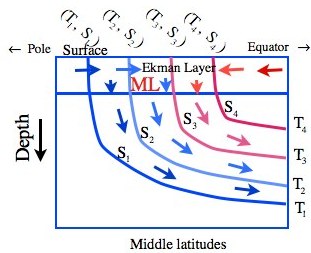
Fig.1.11 Formation of the Central waters at the surface in the Mixed Layer (ML) and their subduction in the middle latitudes. The subducted water slides along the isotherms coinciding with isopycnals to fill the volume of the ocean in the thermocline region. This renewal process is continuous and a necessary component of ocean circulation that enriches the bottom water with oxygen when the water masses come in contact with the atmosphere.